How to Diagnose Latency Using p50, p90, and p99

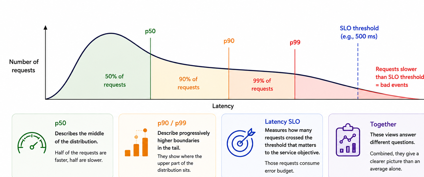
When analyzing latency in application performance monitoring, it is important to consider more than just the average response time. Different percentiles, such as p50, p90, and p99, provide valuable insights into the distribution of latency across requests. These percentiles help identify whether the slowdown is affecting a majority of requests or just a small portion of the workload.

The p50 percentile, also known as the median, represents the latency around the middle of the distribution. If the p50 value increases, it indicates that the midpoint of the distribution has shifted, meaning that the majority of requests are experiencing longer latencies. This is useful for identifying changes that affect common request paths or shared resources, such as CPU pressure, database slowdowns, or connection pool issues.

In contrast, the p90 percentile describes a boundary closer to the slower part of the distribution. If the p90 value increases while the p50 remains relatively stable, it suggests that the slower portion of the workload has changed, while the middle of the distribution has not moved as significantly. This pattern can occur when different categories of requests experience different levels of performance degradation, such as cache misses or route-specific issues.

The p99 percentile sits even further into the tail of the distribution. A rise in the p99 value indicates that the far tail of the distribution has shifted, often revealing issues that occur infrequently but still impact a small percentage of requests. These could include problems with unhealthy replicas, occasional garbage collection pauses, or other rare but impactful events.

When all three percentiles (p50, p90, and p99) increase together, it suggests a broad rightward shift in the latency distribution. This can be caused by various factors, such as shared dependencies, CPU or memory pressure, database latency, or deployment changes affecting the majority of requests.

On the other hand, if the p50 remains stable while p90 and p99 increase, the problem is concentrated further into the distribution. This could indicate that the slowdown is primarily affecting a subset of requests, such as those routed to specific instances, tenants, or operations.

Conversely, if p50 and p90 remain relatively stable while p99 rises, the issue is likely concentrated in the far tail of the distribution. This might point to specific problems like replica-specific issues, garbage collection pauses, retries, lock contention, hot keys, or overloaded shards.

An interesting pattern to watch for is when systems approach saturation. As utilisation increases, queueing delay tends to rise non-linearly, causing the slower requests to accumulate additional waiting time. This can result in movement in p99 before p90 and p50, indicating that the tail of the distribution is being impacted before the median changes significantly.

When percentiles are derived from Prometheus histograms, it is important to note that these are estimates based on bucket counts rather than exact latency values. Prometheus histograms record how many observations fall below each configured bucket boundary, but they do not retain the individual latency values. This means that the calculated percentiles are approximations and may not capture subtle variations in latency.

In summary, understanding the relationships between p50, p90, and p99 is crucial for diagnosing latency issues in application performance monitoring. By analyzing these percentiles together, developers and operations teams can gain a more comprehensive view of the latency distribution, identify the specific areas impacted, and take targeted actions to improve overall system performance.